-
Although general relativity (GR) is unquestionably one of the most elegant and effective theories in physics, its position has been called into question by recent observational data [1]. Perhaps the most significant observation is the fast expansion of our universe in early and late times [2−12], which defies explanation within the framework of GR. A variety of theories different from GR have been developed as a result of this discrepancy between theory and observations; these theories are collectively referred to as modified gravity [13]. We have demonstrated that the pursuit of a viable substitute has been beneficial and constructive for our understanding of gravity. Many different types of modified gravities exist, among them the metric
$ f(R) $ theories, metric-affine (Palatini)$ f(R) $ gravity [14−16], teleparallel$ f(T) $ gravities [17, 18], symmetric teleparallel$ f(Q) $ [19−22], and scalar-tensor theories [23, 24]. Naturally, the choice of alterations is very much a question of personal preference. From our perspective, intriguing and highly motivating alternatives are those that provide a more general connection than the typical Levi-Civita one, thus extending the fundamental geometry of spacetime. If no a priori limits are imposed on the connection, the space will usually not be Riemannian [25] and will have both torsion and non-metricity. We conceptualize it as an additional fundamental field overlaying the metric. Identifying the affine relationship allows for the calculation of the final geometric quantities. Metric-affine gravity theories have been developed on this non-Riemannian manifold [26]. Recently, [27] discussed$ f(R) $ gravity theories with a symmetric connection that is torsion-free. These are also known as Palatini$ f(R) $ theories of gravity. U4 theories are$ f(R) $ theories of gravity with torsion but without non-metricity. The dynamics of metric-affine gravity theories were discussed in [28], and the dynamics of generalized Palatini gravity theories were studied in [29]. In [30], metric-affine variational principles in GR were discussed. Most recently, in [31], the role of non-metricity in metric-affine theories of gravity was studied into [32].The metric-affine technique [16−47] has received significant attention in recent years, particularly for its cosmological applications [48−59]. This interest may stem from the straightforward geometrical interpretation of the additional impacts that operate in this framework (in comparison to GR). In other words, spacetime torsion and non-metricity alone are responsible for the alterations. Moreover, matter with inherent structure excites these geometric concepts, as presented in [50] and [60−63]. The MAG scheme gains an additional favorable aspect from this relationship between generalized geometry and inner structure.
This, in turn, gives us a reason to develop cosmological models in these affinely connected metric theories, especially from their Riemann-Cartan subclass [64], using a certain but not unique connection. By creating both non-zero curvature and non-zero torsion at the same time, this would add the extra degrees of freedom that are usually needed for any gravitational change [65]. As a result, both the early and late universe evolution may be satisfactorily explained by metric-affine gravity [66−70]. [66] is a new study of cosmology that was made possible by using this type of framework and computing how observable quantities, such as density parameters and the effective dark energy equation-of-state parameter, change over time. The authors explored the cosmological behavior, emphasizing the connection effect, using the mini-super-space technique and expressing the theory as a deformation from both GR and its teleparallel counterpart. The observational limitations on metric-affine
$ F(R,T) $ gravity were studied by [71]. Several metric-affine gravity theories and their applications were discussed in [72−78].Motivated by the above discussions, we developed some Friedmann-Lemaître-Robertson-Walker (FLRW) cosmological models in torsion-free metric-affine geometry. We recently investigated transit phase cosmological models in metric-affine
$ F(R,T) $ gravity with observational constraints [79]. In [80, 81], we looked into some exact cosmological models in this metric-affine$ F(R,T) $ gravity. In this study, we investigated some FLRW cosmological models and their properties in the metric-affine$ F(R,Q) $ gravity theory. For this purpose, we considered the arbitrary function$ F(R,Q) = R+\lambda Q+\lambda_{0} $ , where R is the Ricci scalar curvature, Q is the non-metricity scalar with respect to non-special connection, and$ \lambda, \lambda_{0} $ are arbitrary constants.The organization of the present paper is as follows: Sec. II presents some geometrical concepts of the metric-affine spacetime. Sec. III provides a brief introduction to the metric-affine
$ F(R,Q) $ gravity. We obtained the gravity field equations from the$ F(R,Q) $ gravity theory and used them to study cosmological field equations of$ F(R,Q) $ gravity in a flat FLRW spacetime in Sec. IV. In Sec. V, we obtained two exact solutions of the derived field equations for different choices of u and w. We imposed observational constraints on the models, obtained using two recent datasets, the$ H(z) $ and Pantheon SNe Ia datasets, by applying a Markov chain Monte Carlo (MCMC) analysis in Sec. VI. Sec. VII explores the results, and Sec. VIII presents the conclusions. -
The notion of metric-affine gravity is a generalization of the underlying connection. In this work, we generalize the connection in such a way that the torsion tensor
$ T_{\,\,\,\, \mu \nu}^{\alpha} $ should vanish (Weyl-type geometry). Therefore, such a connection can be defined as [31]$ \Gamma^{\rho}_{\,\,\,\,\mu\nu} = \breve{\Gamma}_{\,\,\,\, \mu \nu}^{\rho}+L^{\rho}_{\,\,\,\,\mu\nu}, $

(1) where
$ \Gamma^{\rho}_{\,\,\,\,\mu\nu} $ is called the symmetric general affine connection,$ \breve{\Gamma}_{\,\,\,\, \mu \nu}^{\rho} $ is the Levi–Civita connection, and$ L^{\rho}_{\,\,\,\,\mu\nu} $ is the disformation tensor. These two tensors have the following forms:$ \breve{\Gamma}^l_{\, \, \, jk} = \frac{1}{2} g^{lr} \left( \partial _k g_{rj} + \partial _j g_{rk} - \partial _r g_{jk} \right), $

(2) $ L^{\rho}_{\,\,\,\,\mu\nu} = \frac{1}{2}g^{\rho\lambda}\bigl(-Q_{\mu \nu \lambda}-Q_{\nu \mu \lambda} + Q_{\lambda\mu\nu}\bigr) = L^{\rho}_{\,\,\,\,\nu\mu}. $

(3) Here,
$ Q_{\rho \mu \nu} = \nabla_{\rho} g_{\mu \nu} $ is the nonmetricity tensor.Hence, we can express the Ricci curvature tensor
$ R_{\mu\nu} $ in terms of the symmetric metric-affine connection [74, 82, 83] as follows:$ R_{\mu\nu} = \partial_{\lambda}\Gamma^{\lambda}_{\mu\nu}-\partial_{\mu}\Gamma^{\lambda}_{\lambda\nu}+\Gamma^{\lambda}_{\lambda\alpha}\Gamma^{\alpha}_{\mu\nu}-\Gamma^{\lambda}_{\mu\alpha}\Gamma^{\alpha}_{\lambda\nu}, $

(4) or
$\begin{aligned}[b] R_{\mu\nu} =& \breve{R}_{\mu\nu}+\partial_{\lambda}L^{\lambda}_{\mu\nu}-\partial_{\mu}L^{\lambda}_{\lambda\nu}+\breve{\Gamma}^{\lambda}_{\lambda\alpha}L^{\alpha}_{\mu\nu}+\breve{\Gamma}^{\alpha}_{\mu\nu}L^{\lambda}_{\lambda\alpha}\\&-\breve{\Gamma}^{\lambda}_{\mu\alpha}L^{\alpha}_{\lambda\nu}-\breve{\Gamma}^{\alpha}_{\lambda\nu}L^{\lambda}_{\mu\alpha}+L^{\lambda}_{\lambda\alpha}L^{\alpha}_{\mu\nu}-L^{\lambda}_{\mu\alpha}L^{\alpha}_{\lambda\nu},\end{aligned} $

(5) where
$ \breve{R}_{\mu\nu} $ is the Ricci curvature tensor with respect to Levi-Civita connection$ \breve{\Gamma} $ . Now, the Ricci scalar R with respect to the general symmetric metric-affine connection Γ can be expressed as$ R = \breve{R}+u, $

(6) where
$u = u(\Gamma^{\rho}_{\,\,\,\,\mu\nu}, x_i, g_{ij}, {\dot g_{ij}},{\ddot g_{ij}}, ... , f_j)$ is a real function.Similarly, we can express the nonmetricity tensor
$ Q_{\rho\mu\nu} $ with respect to the general symmetric metric connection Γ and in the case of the non-coincident gauge formulation (see [82−83]) as$ Q_{\rho\mu\nu} = \partial_{\rho}g_{\mu\nu}-\Gamma^{\lambda}_{\mu\rho}g_{\lambda\nu}-\Gamma^{\lambda}_{\nu\rho}g_{\lambda\mu}, $

(7) or
$ Q_{\rho\mu\nu} = \breve{Q}_{\rho\mu\nu}+(-L^{\lambda}_{\mu\rho}g_{\lambda\nu}-L^{\lambda}_{\nu\rho}g_{\lambda\mu}). $

(8) Hence, the nonmetricity scalar Q can be expressed as
$ Q = \breve{Q}+w, $

(9) where
$w = w(\Gamma^{\rho}_{\,\,\,\,\mu\nu}, x_i, g_{ij}, {\dot g_{ij}},{\ddot g_{ij}}, ... , h_j)$ is a real function.We will now introduce two geometrical scalars.
$ R = g^{\mu\nu}R_{\mu\nu}, $

(10) $ Q = -g^{\mu\nu}(L^{\alpha}_{\beta\mu}L^{\beta}_{\nu\alpha}-L^{\alpha}_{\beta\alpha}L^{\beta}_{\mu\nu}), $

(11) where R is the curvature scalar and Q is the nonmetricity scalar. Here, u may be a function of w.
-
In the present work, we consider the metric-affine
$ F(R,Q) $ gravity [84]. In this paper, we use the definitions and notations of [85], so we present the basic setup rather briefly here and refer the reader to [85] for additional details. The action for$ F(R,Q) $ gravity is described in [84] as$ S = \frac{1}{2\kappa}\int \left[F(R, Q)+2\kappa L_m\right]\sqrt{-g}\; {\rm d}^4x, $

(12) where
$ F(R, Q) $ is an arbitrary function of the Ricci R scalar and the nonmetricity scalar Q, g is the determinant of$ g_{\mu\nu} $ , and$ {\cal{L}}_m $ is the matter Lagrangian density.This is an extension of both the
$ F(R) $ and$ F(Q) $ theories. Indeed, the function$ F = F(R,Q) $ is a generic function of the scalar curvature R (of the general affine connection Γ) and of Q, where Q is the non-metricity scalar. The two independent traces of$ Q_{\alpha\mu\nu} $ are$ Q_{\alpha} = Q_{\alpha }{}^{\mu }{}_{\mu }\,,\quad \tilde{Q}_{\alpha } = Q^{\mu }{}_{\alpha \mu }. $

(13) The invariant non-metricity scalar is defined as a contraction of
$ Q_{\alpha\mu \nu } $ given by$ Q = -Q_{\alpha \mu \nu }P^{\alpha \mu \nu}, $

(14) where
$ P^{\alpha \mu \nu} $ is the non-metricity conjugate given by$ 4P^{\alpha }{}_{\mu \nu } = -Q^{\alpha }{}_{\mu \nu } + 2Q_{(\mu \phantom{\alpha}\nu )}^{\phantom{\mu}\alpha } - Q^{\alpha }g_{\mu \nu } - \tilde{Q}^{\alpha }g_{\mu \nu }-\delta _{(\mu }^{\alpha }Q_{\nu )}\,. $

(15) The metric field equations of the theory read as follows:
$\begin{aligned}[b] & - \frac{1}{2} g_{\mu \nu} F + F_R R_{(\mu \nu)} + F_Q L_{(\mu \nu)} + \hat{\nabla}_\lambda \left(F_Q {J^\lambda}_{(\mu \nu)} \right) \\ & \qquad + g_{\mu \nu} \hat{\nabla}_\lambda \left(F_Q \zeta^\lambda \right) = \kappa T_{\mu \nu} \,, \end{aligned}$

(16) where
$ F_{R} = \dfrac{\partial F}{\partial R} $ ,$ F_{Q} = \dfrac{\partial F}{\partial Q} $ and$ T_{\mu \nu } = -\dfrac{2}{\sqrt{-g}}\dfrac{\delta \left( \sqrt{-g}{\cal{L}}_{m}\right) }{\delta g^{\mu \nu }} $ ,$ \hat{\nabla}_\lambda : = \frac{1}{\sqrt{-g}}(2S_{\lambda}-\nabla_\lambda) $

(17) and
$ \begin{aligned}[b] \ L_{\mu \nu} : =& \dfrac{1}{4} \left[ \left(Q_{\mu \alpha \beta} - 2 Q_{\alpha \beta \mu} \right) {Q_\nu}^{\alpha \beta} + \left( Q_\mu + 2 \tilde{Q}_\mu \right) Q_\nu \right. \\ &\left. + \left( 2 Q_{\mu \nu \alpha} - Q_{\alpha \mu \nu} \right) Q^\alpha \right]- {\Xi^{\alpha \beta}}_\nu Q_{\alpha \beta \mu} - \Xi_{\alpha \mu \beta} {Q^{\alpha \beta}}_\nu \,, \\ {J^\lambda}_{\mu \nu} : = & \sqrt{-g} \left(\dfrac{1}{4} {Q^\lambda}_{\mu \nu} - \dfrac{1}{2} {Q_{\mu \nu}}^\lambda + {\Xi^\lambda}_{\mu \nu} \right) \,, \\ \zeta^\lambda : = & \sqrt{-g} \left( - \dfrac{1}{4} Q^\lambda + \dfrac{1}{2} \tilde{Q}^\lambda \right) \,, \end{aligned} $

(18) where
$ Q_{\lambda \mu \nu} $ is the non-metricity tensor,$ Q_\lambda $ and$ \tilde{Q}_\lambda $ are its trace parts, and$ \Xi_{\lambda \mu \nu} $ is the so-called (non-metricity) "superpotential". The connection field equations are$ \begin{aligned}[b] & {P_\lambda}^{\mu \nu} (F_R) + F_Q \Bigg[ 2 {Q^{[\nu \mu]}}_\lambda - {Q_\lambda}^{\mu \nu} \\& \quad + \left( \tilde{Q}^\nu - Q^\nu \right) \delta^\mu_\lambda + Q_\lambda g^{\mu \nu} + \frac{1}{2} Q^\mu \delta^\nu_\lambda \Bigg] = 0 \,, \end{aligned} $

(19) where
$ {P_\lambda}^{\mu \nu} (F_R) $ is the modified Palatini tensor:$ {P_\lambda}^{\mu \nu} (F_R) : = - \frac{\nabla_\lambda \left(\sqrt{-g} F_R g^{\mu \nu} \right)}{\sqrt{-g}} + \frac{\nabla_\alpha \left( \sqrt{-g} F_R g^{\mu \alpha}\delta^\nu_\lambda \right)}{\sqrt{-g}} \,, $

(20) where
$ \nabla $ is the covariant derivative associated with the general affine connection Γ.We assume that the matter is a perfect fluid whose energy-momentum tensor
$ T_{\mu \nu } $ is given by$ T_{\mu \nu } = (\rho +p)u_{\mu }u_{\nu }+pg_{\mu \nu }\,, $

(21) where
$ u_{\mu } $ is the four-velocity satisfying the normalization condition$ u_{\mu }u^{\mu } = -1 $ , whereas ρ and p are the energy density and pressure of a perfect fluid, respectively. -
First, let us rewrite action (12) as
$ \begin{aligned}[b] S =& \frac{1}{2\kappa^{2}}\int \sqrt{-g}d^{4}x[F(R,Q)\\&-\lambda_{1}(R-R_{s}-u)-\lambda_{3}(Q-Q_{s}-w)+2\kappa^{2}L_{m}]. \end{aligned} $

(22) The variations of the action with respect to
$ R, Q $ give$ \lambda_{1} = F_{R}, \lambda_{3} = F_{Q} $ , respectively. Thus, action (22) takes the form$ \begin{aligned}[b] S =& \frac{1}{2\kappa^{2}}\int \sqrt{-g}{\rm d}^{4}x[F-F_{R}(R-R_{s}-u)-\\&F_{Q}(Q-Q_{s}-w)+2\kappa^{2}L_{m}], \end{aligned} $

(23) where we know from Eqs. (6) and (9) that
$u = u(g_{ij}, \dot{g}_{ij}, \ddot{g}_{ij}, ...), \quad w = w(g_{ij}, \dot{g}_{ij}, \ddot{g}_{ij}, ...)$ . We now consider the FLRW spacetime case with the metric$ {\rm d} s^2 = -N^{2} (t){\rm d}t^2+a^2(t)({\rm d}x^2+{\rm d}y^2+{\rm d}z^2), $

(24) where
$ a = a(t) $ represents the scale factor,$ N(t) $ represents the lapse function, and$ N(t) = 1 $ is assumed. Then, integrating by parts gives the following action with the point-like FLRW Lagrangian:$ S = \frac{1}{2\kappa^{2}}\int {\cal{L}}{\rm d}t. $

(25) The point-like Lagrangian has the form
$ {\cal{L}} = a^{3} [F-F_{R}(R-R_{s}-u)-F_{Q}(Q-Q_{s}-w)+2\kappa^{2}L_{m}]. $

(26) In FLRW spacetime, we have
$ R_{s} = 6(\frac{\ddot{a}}{a}+\frac{\dot{a}^{2}}{a^{2}}) = 6(2H^{2}+\dot{H}), $

(27) $ Q_{s} = 6\frac{\dot{a}^{2}}{a^{2}} = 6H^{2}. $

(28) Finally, we obtain the following FLRW Lagrangian:
$ \begin{aligned} {\cal{L}}(a,R,Q,\dot{a},\dot{R},\dot{Q}) =& a^{3}(F-RF_{R}-QF_{Q})+6a\dot{a}^{2}(F_{R}+F_{Q})\\&+6a^{2}\dot{a}\dot{F}_{R}+a^{3}(uF_{R}+wF_{Q})+2\kappa^{2}a^{3}L_{m}. \end{aligned} $

(29) Now, taking the Hamiltonian
$ {\cal{H}} $ of the Lagrangian$ {\cal{L}} $ as$ {\cal{H}} = {\cal{E}} = \dot{a}\frac{\partial {\cal{L}}}{\partial \dot{a}}+\dot{R}\frac{\partial {\cal{L}}}{\partial \dot{R}}+\dot{Q}\frac{\partial {\cal{L}}}{\partial \dot{Q}}-{\cal{L}} = 0 $

(30) and the Euler-Lagrange equations corresponding to the Lagrangian
$ {\cal{L}} $ , we obtain the following field equations:$\begin{aligned}[b] -\frac{1}{2}(F-&RF_{R}-QF_{Q})+3H^{2}(F_{R}+F_{Q})\\&-\frac{1}{2}\left[(u-\dot{a}u_{\dot{a}})F_{R}+(w-\dot{a}w_{\dot{a}})F_{Q}\right]\\&+3H(\dot{R}F_{RR}+\dot{Q}F_{RQ}) = \kappa^{2}\rho, \end{aligned} $

(31) $ \begin{aligned}[b] -\frac{1}{2}(F-&RF_{R}-QF_{Q})+(2\dot{H}+3H^{2})(F_{R}+F_{Q})\\ &-\frac{1}{2}(u+\frac{1}{3}au_{a}-\dot{a}u_{\dot{a}}-\frac{1}{3}a\dot{u}_{\dot{a}})F_{R}\\ &-\frac{1}{2}(w+\frac{1}{3}aw_{a}-\dot{a}w_{\dot{a}}-\frac{1}{3}a\dot{w}_{\dot{a}})F_{Q}\\ & +2H(\dot{F}_{R}+\dot{F}_{Q})+\frac{1}{6}a(u_{\dot{a}}\dot{F}_{R}+w_{\dot{a}}\dot{F}_{Q})\\ &+\ddot{F}_{R} = -\kappa^{2}p, \end{aligned}$

(32) where
$ \rho = L_{m}-\dot{a}\frac{\partial L_{m}}{\partial \dot{a}},\; \; \; \; p = \frac{1}{3a^{2}}\left[\frac{{\rm{d}}}{{\rm{d}}t}\left(a^{3}\frac{\partial L_{m}}{\partial \dot{a}}\right)-\frac{\partial}{\partial a}(a^{3}L_{m})\right]. $

(33) -
In the present work, we are interested in investigating the cosmological behavior that arises purely from the non-special symmetric connection of metric-affine gravity. We selected the simplest case, where the arbitrary function is simple:
$ F(R,Q) = R+\lambda Q+\lambda_{0} $ . Here, λ is a dimensionless parameter (we do not include the coupling coefficient of R because it can be absorbed into$ \kappa^{2} $ ) and$ \lambda_{0} $ is an arbitrary constant (a model free parameter of dimension of$ H_{0}^{2} $ ). As a result, for this particular case of the arbitrary function$ F(R,Q) = R+\lambda Q+\lambda_{0} $ with$ \lambda, \lambda_{0} $ as model parameters, the field Eqs. (31) and (32) become$ 3(1+\lambda)H^{2}-\frac{1}{2}[(u-\dot{a}u_{\dot{a}})+\lambda(w-\dot{a}w_{\dot{a}})]-\frac{\lambda_{0}}{2} = \kappa^{2}\rho, $

(34) $ \begin{aligned}[b] (1+&\lambda)(2\dot{H}+3H^{2})-\frac{1}{2}[(u+\frac{1}{3}au_{a}-\dot{a}u_{\dot{a}}-\frac{1}{3}a\dot{u}_{\dot{a}})\\&+\lambda(w+\frac{1}{3}aw_{a}-\dot{a}w_{\dot{a}}-\frac{1}{3}a\dot{w}_{\dot{a}})]-\frac{\lambda_{0}}{2} = -\kappa^{2}p. \end{aligned} $

(35) At the same time, for the original density and pressure, the continuity equation takes the form
$ \dot{\rho}+3H(\rho+ p)+\frac{1}{2\kappa^{2}}(\dot{y}-\dot{a}y_{a}-\ddot{a}y_{\dot{a}}) = 0, $

(36) where
$ y = u+\lambda w. $

(37) Now, we have two linearly independent field equations, (34) and (35), in five unknowns:
$ \rho, p, a, u, w $ . To find the exact solutions to these two field equations, we must impose at least three constraints on these unknowns. This modified$ F(R,Q) $ gravity theory depends upon the choices of the factors$ u(a,\dot{a}, \ddot{a},..) $ and$ w(a,\dot{a}, \ddot{a},..) $ , which can be considered as per their definitions (see (6) and (9)). Therefore, we investigate the above model using two different choices for u and w, resulting in two distinct cosmological models, as detailed below. -
As we have discussed in Sec. 2, the scalars u and w may be functions of scale factor
$ a(t) $ , connection Γ, and its derivatives. In our study, we selected the scalars u and w such that the energy conservation equation (36) is satisfied. Thus, to obtain the exact solutions to the field equations (34) and (35), without loss of generality, we can pick$ u = c_{1}\dfrac{\dot{a}}{a}\ln\dot{a} $ and$ w = s(a)\dot{a} $ , where$ c_{1} $ is a constant and$ s(a) $ is any function of a. There may be several such choices as per the concepts of$ u, w $ (see [71, 79−81]). Then, the above field equations (34) and (35) become$ 3(1+\lambda)H^{2}+\frac{1}{2}c_{1}H-\frac{1}{2}\lambda_{0} = \kappa^{2}\rho, $

(38) $ (1+\lambda)(2\dot{H}+3H^{2})+\frac{1}{6}c_{1}\frac{\dot{H}}{H}+\frac{1}{2}c_{1}H-\frac{1}{2}\lambda_{0} = -\kappa^{2}p, $

(39) and the energy conservation equation (36) becomes
$ \dot{\rho}+3H(\rho+ p) = 0, $

(40) As the third constraint, we take matter pressure as
$ p\approx0 $ , and solving the energy conservation equation (40), we obtain the matter energy density ρ as$ \rho = \rho_{0}\left(\frac{a_{0}}{a}\right)^{3} = \rho_{0}(1+z)^{3}, $

(41) where
$ \rho_{0} $ is the present value of energy density ρ at$ z = 0 $ and$ \dfrac{a_{0}}{a} = 1+z $ with$ a(t) $ as scale factor.Now, from (38), we can find the relation at present (
$ z = 0 $ ) as$ 6(1+\lambda) = 6\Omega_{m0}+\frac{\lambda_{0}}{H_{0}^{2}}-\frac{c_{1}}{H_{0}} $

(42) where
$\Omega_{m0} = {\kappa^{2}\rho_{0}}/({3H_{0}^{2}})$ . The Eq. (42) suggests that λ is a dimensionless parameter,$ \lambda_{0} $ is a parameter of dimension$ H_{0}^{2} $ , and$ c_{1} $ is a parameter of dimension$ H_{0} $ , because$ \Omega_{m0} $ is a well-defined dimensionless cosmological parameter in cosmology. Using Eqs. (41) and (42) in Eq. (38), we can obtain the Hubble function as$ H(z) = \dfrac{2H_{0}\left[\dfrac{\lambda_{0}}{H_{0}^{2}}+6\Omega_{m0}(1+z)^{3}\right]}{\dfrac{c_{1}}{H_{0}}+\sqrt{\left(\dfrac{c_{1}}{H_{0}}\right)^{2}+4\left(6\Omega_{m0}+\dfrac{\lambda_{0}}{H_{0}^{2}}-\dfrac{c_{1}}{H_{0}}\right)\left[\dfrac{\lambda_{0}}{H_{0}^{2}}+6\Omega_{m0}(1+z)^{3}\right] }}, $ 
(43) where
$ \Omega_{m0} $ denotes the present value of the corresponding parameter, and$ H_{0} $ is the Hubble constant.Now, Eqs. (38) and (39) can be rewritten as equivalent to Friedmann equations.
$ 3H^{2} = \kappa^{2}\rho+\kappa^{2}\rho_{de}, $

(44) $ 2\dot{H}+3H^{2} = -\kappa^{2}p-\kappa^{2}p_{de}, $

(45) where
$ \rho_{de} $ and$ p_{de} $ , energy density and pressure, are derived from geometrical modifications and are given, respectively, as$ \rho_{de} = \frac{1}{2\kappa^{2}}\left[\lambda_{0}-c_{1}H-6\lambda H^{2}\right], $

(46) $ p_{de} = -\frac{1}{6\kappa^{2}}\left[3\lambda_{0}-3c_{1}H-18\lambda H^{2}-12\lambda \dot{H}-c_{1}\frac{\dot{H}}{H}\right]. $

(47) Therefore, we derive the effective dark equation of state as
$ \omega_{de} = -1-\frac{(c_{1}+12\lambda H)(1+z)H'}{3\lambda_{0}-3c_{1}H-18\lambda H^{2}}. $

(48) Now, we can derive the deceleration parameter
$ q(z) $ from Eq. (43) as$ q(z) = -1+(1+z)\frac{H'}{H} $

(49) where
$H' = \dfrac{{\rm d}H}{{\rm d}z}$ . -
In this model, we adopted
$ u = c_{2}\dfrac{\ddot{a}}{a} $ as a function of the second derivative of a and$ w = c_{3}\dot{a} $ as a function of the first derivative of a, with$ c_{2} $ ,$ c_{3} $ as constants such that the energy conservation equation (36) is satisfied. However, there may be several such choices as per the concepts of$ u, w $ (see [71, 79−81]). Now, using these expressions of u and w in Eqs. (34) and (35), we obtain the following simplified field equations:$ -\frac{c_{2}}{2}\dot{H}+\frac{6(1+\lambda)-c_{2}}{2}H^{2}-\frac{\lambda_{0}}{2} = \kappa^{2}\rho, $

(50) $ \frac{6(1+\lambda)-c_{2}}{3}\dot{H}+\frac{9(1+\lambda)-c_{2}}{3}H^{2}-\frac{\lambda_{0}}{2} = -\kappa^{2}p, $

(51) and the energy conservation equation (36) reduces to
$ \dot{\rho}+3H(\rho+ p) = 0. $

(52) Applying the third constraint on matter pressure as
$ p = 0 $ , and using Eq. (41) in (50) and (51), we obtain the Hubble function as$ H(z) = H_{0}\sqrt{1+\frac{2(6+6\lambda-c_{2})}{(1+\lambda)(12+12\lambda-c_{2})}\Omega_{m0}[(1+z)^{3}-1]},\, $

(53) where
$ \frac{2\lambda_{0}(c_{2}+3+3\lambda)}{3(1+\lambda)(12+12\lambda-c_{2})}+\frac{2(6+6\lambda-c_{2})}{(1+\lambda)(12+12\lambda-c_{2})} = 1.\, $

(54) Now, Eqs. (50) and (51) can be rewritten as equivalent to Friedmann equations
$ 3H^{2} = \kappa^{2}\rho+\kappa^{2}\rho_{de}, $

(55) $ 2\dot{H}+3H^{2} = -\kappa^{2}p-\kappa^{2}p_{de}, $

(56) where the effective energy density
$ \rho_{de} $ and pressure$ p_{de} $ are derived from a geometrical modification in the Einstein's field equations, and are expressed as$ \rho_{de} = \frac{1}{2\kappa^{2}}\left[\lambda_{0}+(c_{2}-6\lambda)H^{2}+c_{2}\dot{H}\right], $

(57) $ p_{de} = -\frac{1}{6\kappa^{2}}\left[3\lambda_{0}+2(c_{2}-9\lambda)H^{2}+2(c_{2}-6\lambda)\dot{H}\right]. $

(58) Hence, the effective dark equation of state is derived as
$ \omega_{de} = -1+\frac{c_{2}H^{2}-(c_{2}+12\lambda)(1+z)HH'}{3[\lambda_{0}+(c_{2}-6\lambda)H^{2}-c_{2}(1+z)HH']}. $

(59) Using Eq. (53), we derive the deceleration parameter as
$ q(z) = -1+\dfrac{\dfrac{3(6+6\lambda-c_{2})}{(1+\lambda)(12+12\lambda-c_{2})}\Omega_{m0}(1+z)^{3}}{1+\dfrac{2(6+6\lambda-c_{2})}{(1+\lambda)(12+12\lambda-c_{2})}\Omega_{m0}[(1+z)^{3}-1]}. $

(60) -
In this part, we utilize observational datasets to provide constraints on the model parameters in our derived model. To accomplish this, we utilize the Emcee software, which is readily accessible at [86], to conduct an MCMC analysis. This allows us to compare our generated model with observational datasets. The MCMC sampler restricts the cosmological and model parameters by varying their values within a plausible range of prior distributions and examining the resulting posterior distributions in the parameter space. In this section, we assess the compatibility between the solution in the model and the cosmic chronometer (CC) data and Pantheon datasets. These datasets are related to the observed universe at a recent time frame.
-
The Hubble parameter holds significant importance for both theoretical and observational cosmologists as it is a crucial cosmological parameter for investigating the progression of the universe. Observed values for Hubble datasets
$ H(z) $ can be found for different redshifts z. To determine the optimal values for model parameters, taking into account the uncertainty range of redshift ($ 0.07 \leqslant z \leqslant 1.965 $ ), we employ an MCMC simulation. This simulation allows us to compare the Hubble function derived from the field equations with the observed values of the 31 CC data points (referred to as Hubble data) [87−89]. The values were determined using the differential ages (DA) of galaxies approach. To estimate the model parameters$ H_{0} $ ,$ \Omega_{m0} $ ,$ c_{1} $ ,$ c_{2} $ and$ \lambda_{0} $ , λ, we can minimize the$ \chi^{2} $ function, which is equivalent to maximizing the likelihood function. The expression for the$ \chi^{2} $ function is$ \chi_{CC}^{2}(\phi) = \sum\limits_{i = 1}^{i = N}\frac{[H_{ob}(z_{i})-H_{th}(\phi, z_{i})]^{2}}{\sigma_{H(z_{i})}^{2}}, $

Here, N denotes the total amount of data,
$ H_{ob},\; H_{th} $ , respectively, the observed and hypothesized datasets of$ H(z) $ , and the standard deviations are expressed by$ \sigma_{H(z_{i})} $ . Here,$\phi = (H_{0}, \;\Omega_{m0}, \;c_{1}, \;\lambda_{0})$ for Model-I, and$\phi = (H_{0}, \Omega_{m0}, \;\lambda,\; c_{2})$ for Model-II.We employed Bayesian statistical analysis for the MCMC simulation to calibrate the CC datasets. To achieve this, we used the Emcee package developed by Foreman-Mackey et al. [86]. We reduced the chi-squared statistic,
$ \chi_{CC}^{2}(\phi) $ , in order to find the best values for the model's parameters. Table 1 presents the values.Model Parameter Prior Value Model-I $ H_{0} $ 

$ (40,100) $ 

$ 68.9_{-2.6}^{+3.0} $ 

$ \Omega_{m0} $ 

$ (0, 0.6) $ 

$ 0.42_{-0.10}^{+0.14} $ 

$ \lambda_{0} $ 

$ (10000, 60000) $ 

$ 28460\pm10000 $ 

$ c_{1} $ 

$ (0, 2) $ 

$ 0.98_{-0.66}^{+0.57} $ 

$\chi_{\min}^{2}$ 

– $ 14.493 $ 

Model-II $ H_{0} $ 

$ (40,100) $ 

$ 68.3\pm2.6 $ 

$ \Omega_{m0} $ 

$ (0, 0.6) $ 

$ 0.445\pm0.090 $ 

λ $ (0, 1) $ 

$ 0.54\pm0.28 $ 

$ c_{2} $ 

$ (-3, 0) $ 

$ -2.03\pm0.58 $ 

$\chi_{\min}^{2}$ 

– $ 14.494 $ 

ΛCDM $ H_{0} $ 

$ (40,100) $ 

$ 67.7\pm3.1 $ 

$ \Omega_{m0} $ 

$ (0, 1) $ 

$ 0.333_{-0.07}^{+0.05} $ 

$\chi_{\min}^{2}$ 

– $ 14.494 $ 

Table 1. Markov chain Monte Carlo (MCMC) results in
$ H(z) $ dataset analysis. -
The correlation between luminosity distance and redshift is a fundamental observational method employed to monitor the progression of the cosmos. When calculating the luminosity distance (
$ D_{L} $ ) in relation to the cosmic redshift (z), the expansion of the universe and the redshift of light from distant bright objects are factored in. It is given as$ D_{L} = a_{0} r (1+z), $

(61) where the radial coordinate of the source r is established by
$ r = \int^r_{0}{\rm d}r = \int^t_{0}\frac{c{\rm d}t}{a(t)} = \frac{1}{a_{0}}\int^z_0\frac{c{\rm d}z'}{H(z')}, $

(62) where we have used
$ {\rm d} t = {\rm d} z/\dot{z}, \dot{z} = -H(1+z) $ .Consequently, the following formula determines the luminosity distance:
$ D_{L} = c(1+z)\int^z_0\frac{{\rm d}z'}{H(z')}. $

(63) Supernovae (SNe) are commonly employed by researchers as standard candles to investigate the pace of cosmic expansion using the reported apparent magnitude (
$ m_{o} $ ). The surveys on supernovae that discovered several types of supernovae of varying magnitudes resulted in the creation of the Pantheon sample SNe datasets, comprising$ 1048 $ data points within the range of$ 0.01 $ to$ 2.26 $ for the variable z. The theoretical apparent magnitude (m) of these standard candles is precisely defined as [90]$ m(z) = M+ 5\; \log_{10}\left(\frac{D_{L}}{Mpc}\right)+25, $

(64) where M represents the absolute magnitude. The luminosity distance is quantified in units of distance. The Hubble-free luminosity distance (
$ d_{L} $ ) can be expressed as$d_{L}\equiv{H_{0}}D_{L}/{c}$ , where$ D_{L} $ is a dimensionless quantity based on$ D_{L} $ . Therefore, we can express$ m(z) $ in a simplified form as shown below$ m(z) = M+5\log_{10}{d_{L}}+5\log_{10}\left(\frac{c/H_{0}}{Mpc}\right)+25. $

(65) The equation provided allows for the observation of the degeneracy between M and
$ H_{0} $ , which remains constant in the Lambda cold dark matter (ΛCDM) background [90, 91]. By redefining, we can combine these deteriorated parameters.$ {\cal{M}}\equiv M+5\log_{10}\left(\frac{c/H_{0}}{Mpc}\right)+25. $

(66) The dimensionless parameter
$ {\cal{M}} $ is defined by the equation$ {\cal{M}} = M-5\log_{10}(h)+42.39 $ , where$ H_{0} $ is equal to$h\times100~ {\rm Km/s/Mpc}$ . In the MCMC analysis, we utilize this parameter in conjunction with the appropriate$ \chi^{2} $ value for the Pantheon data, as provided in [92].$ \chi^{2}_{P} = V_{P}^{i}C_{ij}^{-1}V_{P}^{j} \, . $

(67) The expression
$ V_{P}^{i} $ is defined as the difference between$ m_{o}(z_{i}) $ and$ m(z) $ . The matrix$ C_{ij} $ is the inverse of the covariance matrix, and the value of$ m(z) $ is determined by Eq. (65).Statistical Analysis:
This section examines several cosmological theories using the Akaike information criterion (AIC) and Bayesian information criterion (BIC). Furthermore, we calculate the reduced chi-squared value by employing the method (
$\chi_{\rm red}^{2} = \chi^{2}_{\rm min}/dof$ ), where "dof" denotes the degrees of freedom. We commonly determine the degrees of freedom by subtracting the number of fitted parameters from the number of data points used. For elucidation purposes, however, it is advisable to exclusively employ the$\chi^{2}_{\rm min}/dof$ metric, as the degrees of freedom may not be apparent for models that do not exhibit linearity in relation to the independent parameters [93]. The AIC, which is based on information theory, acts as an estimator of asymptotically unbiased Kullback-Leibler information. The AIC can be approximated using the formula stated in references [94, 95], assuming Gaussian errors.$ AIC = -2\ln({\cal{L}}_{\rm max})+2n+\frac{2n(n+1)}{N-n-1}. $

(68) The symbol
${\cal{L}}_{\rm max}$ denotes the maximum likelihood of the dataset(s) being analyzed. The variable N reflects the total number of data points used in the analysis, whereas n represents the number of fitted parameters. Maximizing the likelihood function is synonymous with minimizing the$ \chi^{2} $ value. When N is a big value, it is clear that this expression produces the original version of AIC, which can be approximated as$AIC\backsimeq-2\ln({\cal{L}}_{\rm max})+2n$ . As stated in the discussion in [96], the utilization of the modified AIC is usually considered the most effective strategy. The BIC is a Bayesian evidence estimator, and it is cited by [94−96].$ BIC = -2\ln({\cal{L}}_{\rm max})+n\ln(N) $

(69) Our goal is to organize the models according to their ability to accurately correspond to the given data, taking into account a set of scenarios that portray the same type of occurrence. To determine the disparity in the values of the information criteria (IC) for a given collection of models, we employ the two IC mentioned before. The expression
$\Delta IC_{\rm model} = IC_{\rm model}-IC_{\rm min}$ represents the difference between a model's IC value ($IC_{\rm model}$ ) and the model's IC value with the lowest IC value ($IC_{\rm min}$ ). To assess the appropriateness of each model, we employ the Jeffreys scale [97]. Specifically, when the value of$ \Delta IC $ is less than or equal to 2, it signifies that the data provides significant evidence in favor of the most preferred model. When the difference between IC values is between 2 and 6, it indicates a considerable amount of disagreement between the two models. Finally, when the difference in IC is greater than or equal to 10, it indicates a significant degree of tension between the models [71].Our approach incorporates two distinct datasets: the CC (Hubble data) points and the Pantheon SNe Ia datasets. The model parameters for our derived models were fitted by minimizing the
$ \chi^{2} $ value. The resulting values of$\chi_{\rm min}^{2}$ are presented in Tables 1 and 2, respectively. For models I and II, we calculated the minimum chi-square value ($\chi_{\rm min}^{2} = 14.493, 14.494$ ), respectively, using CC datasets, whereas for ΛCDM$ \chi^{2} = 14.494 $ . We also determined the AIC and BIC values, which are presented in Table 3, along with the difference from the best-fitted model ($\Delta IC_{\rm model} = IC_{\rm model}- IC_{\rm min}$ ). The total number of data points is$ N = 31 $ and the number of parameters is$ n = 4 $ for models I and II, whereas for ΛCDM$ n = 2 $ .Model Parameter Prior Value Model-I $ H_{0} $ 

$ (40,100) $ 

$ 81.0\pm10 $ 

$ \Omega_{m0} $ 

$ (0, 0.6) $ 

$ 0.43\pm0.11 $ 

$ \lambda_{0} $ 

$ (10000, 60000) $ 

$ 40020\pm10000 $ 

$ {\cal{M}} $ 

$ (23, 24) $ 

$ 23.806\pm0.011 $ 

$ c_{1} $ 

$ (0, 2) $ 

$ 0.94\pm0.55 $ 

$\chi_{\rm min}^{2}$ 

– $ 1026.670 $ 

Model-II $ \Omega_{m0} $ 

$ (0, 0.6) $ 

$ 0.441_{-0.078}^{+0.087} $ 

λ $ (0, 1) $ 

$ 0.62_{-0.24}^{+0.30} $ 

$ {\cal{M}} $ 

$ (23, 24) $ 

$ 23.809\pm0.010 $ 

$ c_{2} $ 

$ (-3, 0) $ 

$ -2.02\pm0.55 $ 

$\chi_{\rm min}^{2}$ 

– $ 1026.671 $ 

ΛCDM $ \Omega_{m0} $ 

$ (0, 1) $ 

$ 0.300\pm0.021 $ 

$ {\cal{M}} $ 

$ (23, 24) $ 

$ 23.810\pm0.011 $ 

$\chi_{\rm min}^{2}$ 

– $ 1026.671 $ 

Table 2. MCMC results in Pantheon SNe Ia dataset analysis.
Model AIC ΔAIC BIC ΔBIC Model-I $ 24.032 $ 

$ 5.110 $ 

$ 28.229 $ 

$ 6.868 $ 

Model-II $ 24.032 $ 

$ 5.110 $ 

$ 28.230 $ 

$ 6.868 $ 

ΛCDM $ 18.922 $ 

$ 0 $ 

$ 21.362 $ 

$ 0 $ 

Table 3. Akaike information criterion (AIC) and Bayesian information criterion (BIC) for the examined cosmological models along cosmic chronometer (CC) datasets.
We used
$ \chi^{2} = 1026.670 $ ,$ N = 1048 $ , and$ n = 5 $ for Model-I, and$ \chi^{2} = 1026.671 $ ,$ N = 1048 $ , and$ n = 4 $ for Model-II, whereas for ΛCDM, we used$ \chi^{2} = 1026.671 $ ,$ N = 1048 $ , and$ n = 2 $ to obtain the AIC and BIC values for the Pantheon SNe Ia datasets. The AIC and BIC values are listed in Table 4, along with the difference from the best-fitting model, which is$\Delta IC_{\rm model} = IC_{\rm model}-IC_{\rm min}$ .Model AIC ΔAIC BIC ΔBIC Model-I $ 1036.728 $ 

$ 6.046 $ 

$ 1061.443 $ 

$ 20.863 $ 

Model-II $ 1034.709 $ 

$ 4.027 $ 

$ 1054.489 $ 

$ 13.909 $ 

ΛCDM $ 1030.682 $ 

$ 0 $ 

$ 1040.580 $ 

$ 0 $ 

Table 4. AIC and BIC for the examined cosmological models along Pantheon SNe Ia datasets.
-
Based on the findings presented in the previous section, we proceed to examine FLRW cosmological models under metric-affine
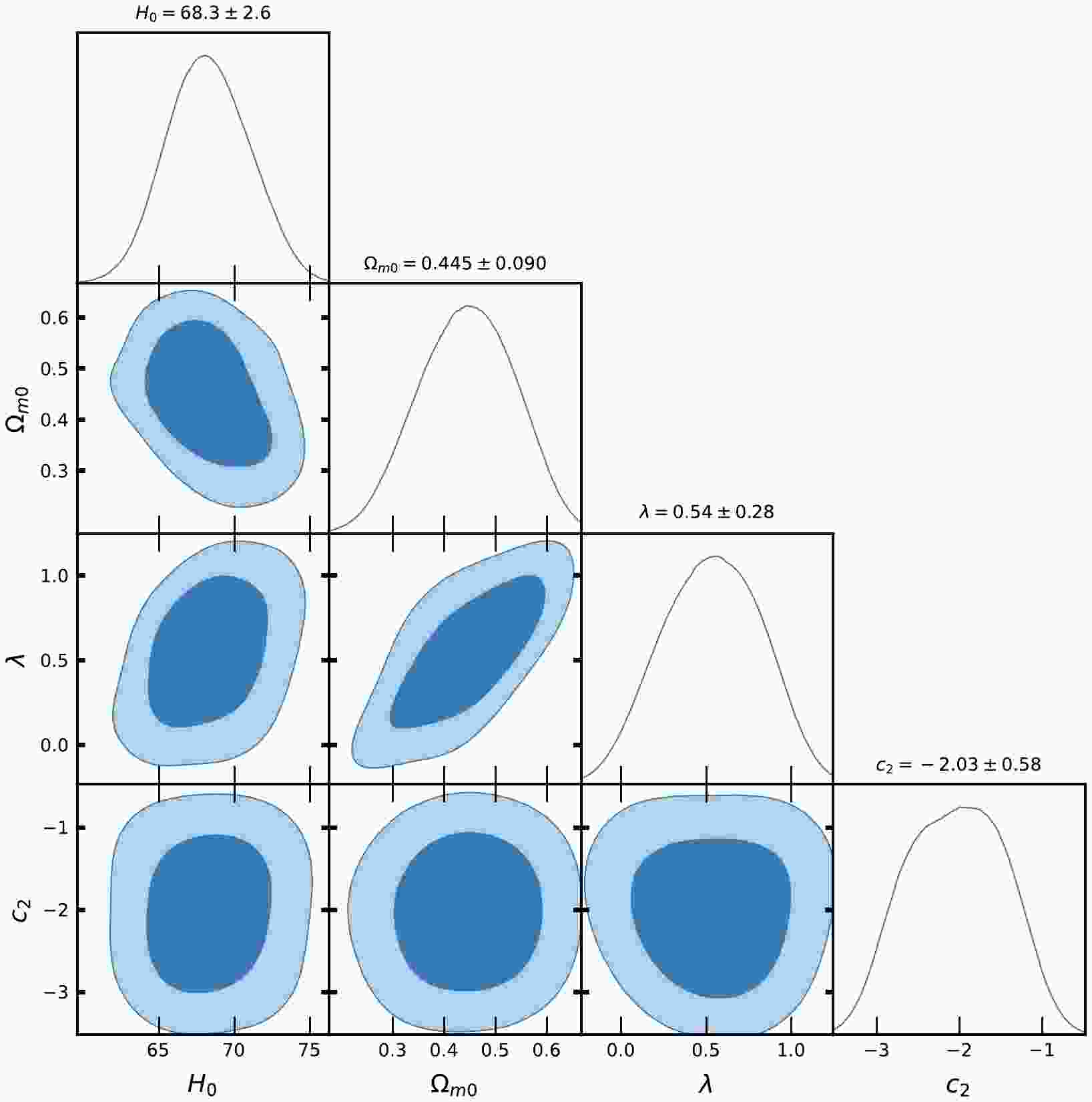
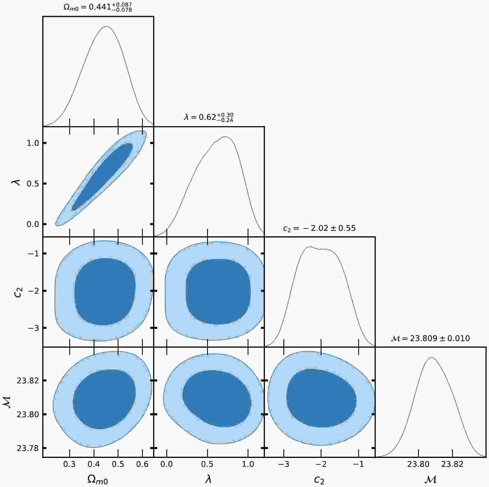
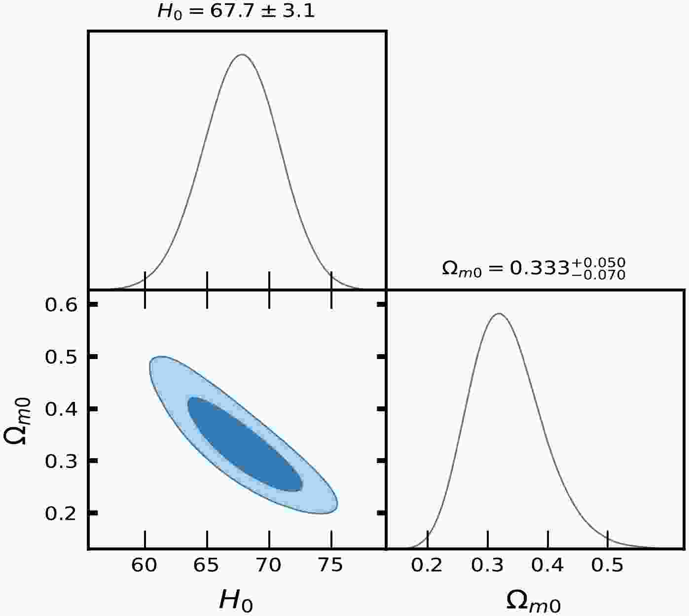
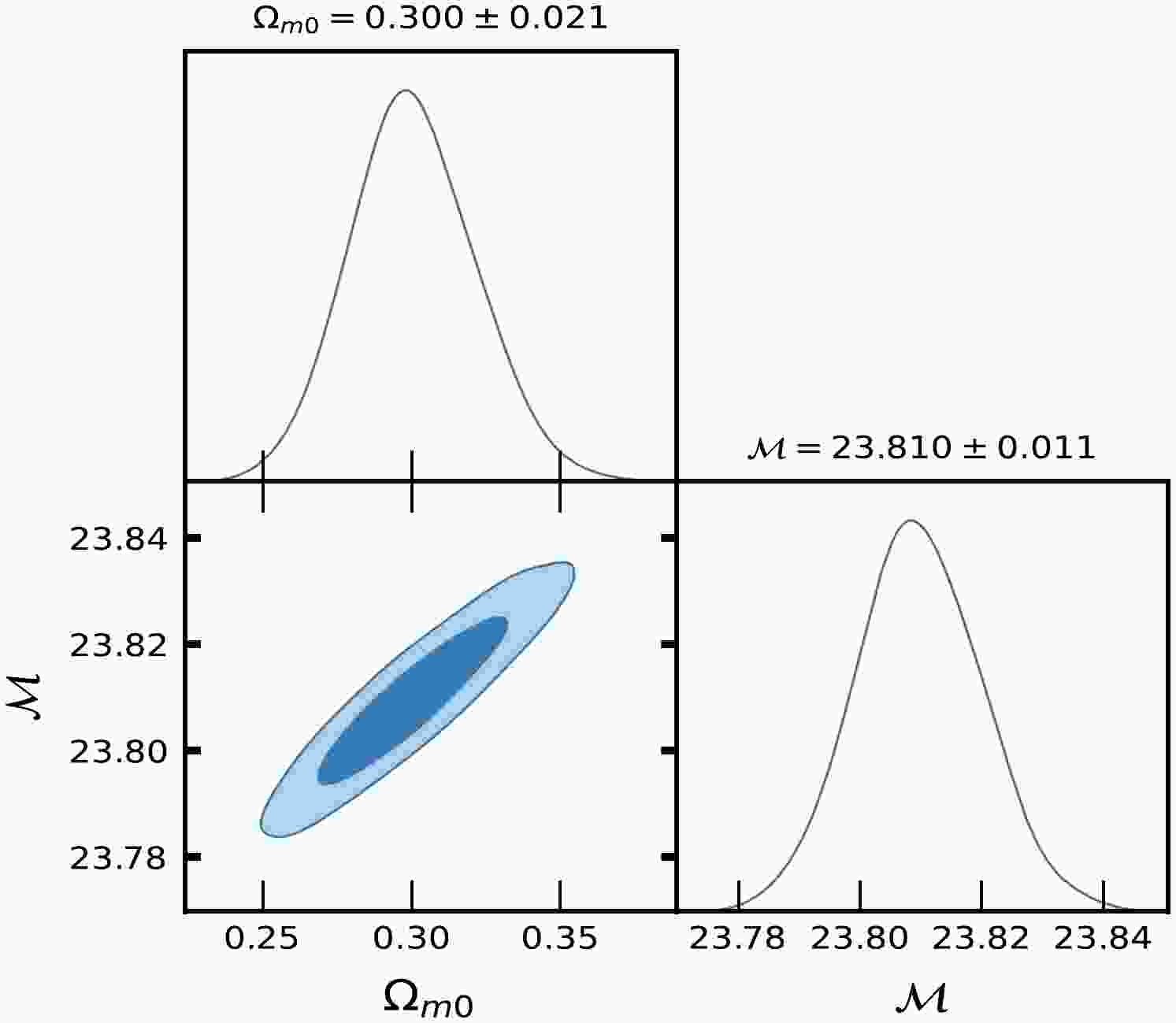
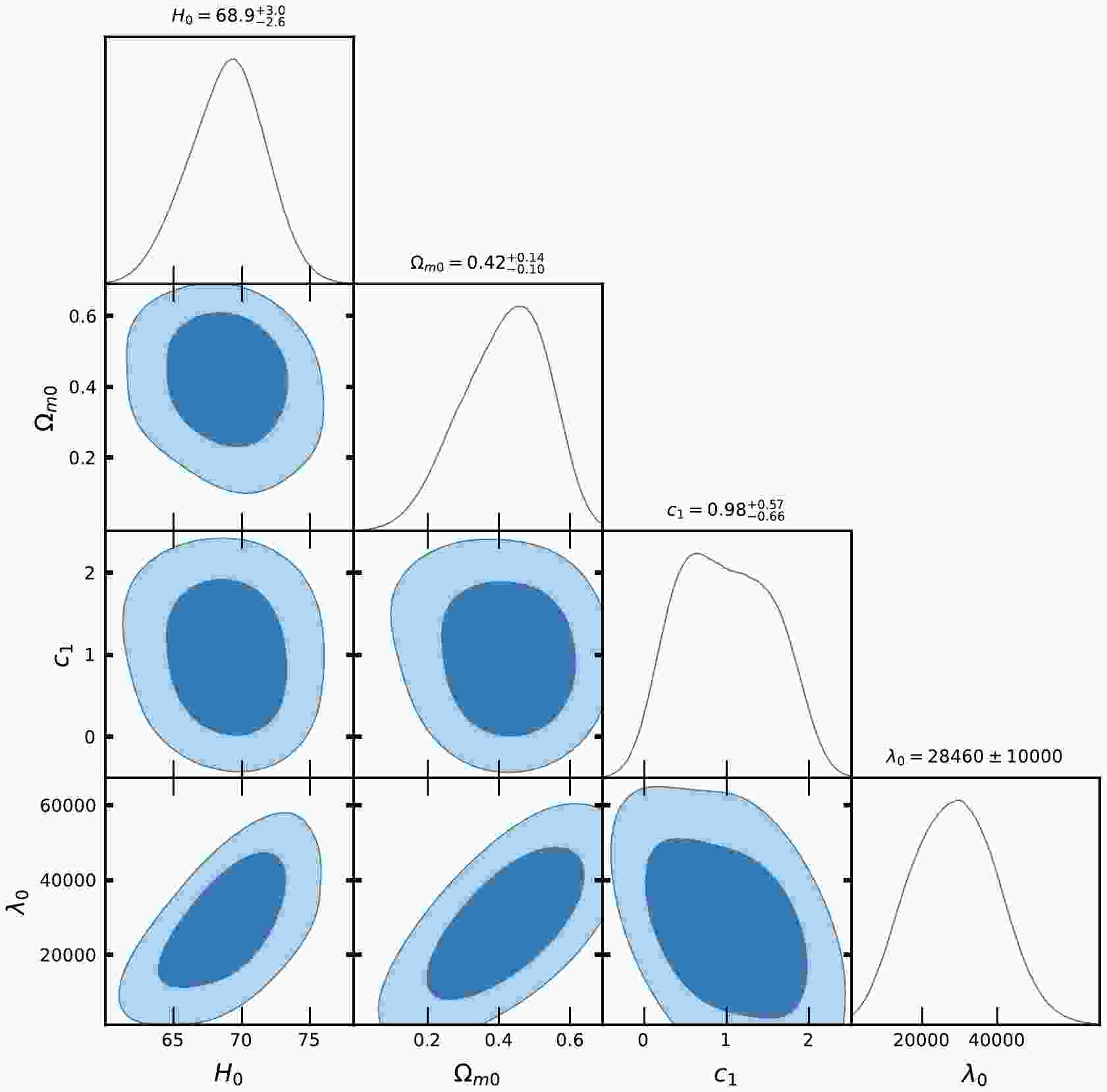
$ F(R,Q) $ gravity from an observational perspective. It is important to emphasize that the models stated above have some parameters that are free to be determined. These parameters include$ H_{0} $ ,$ \Omega_{m0} $ , λ,$ \lambda_{0} $ ,$ c_{1} $ , and$ c_{2} $ . However, in the case of concordance cosmology, the only free parameters are$ H_{0} $ ,$ \Omega_{m0} $ . To enhance convenience, we compile the acquired outcomes in Tables 1 and 2. In addition, we provide contour plots for Model-I and Model-II in Figs. 1, 2, 4, and 5, respectively. In addition, we examined the concordance model, namely, the ΛCDM model, to compare and establish a standard for evaluation. Figures 3 and 6 depict the contour plots for ΛCDM corresponding to the two observational datasets, CC and Pantheon SNe Ia, respectively.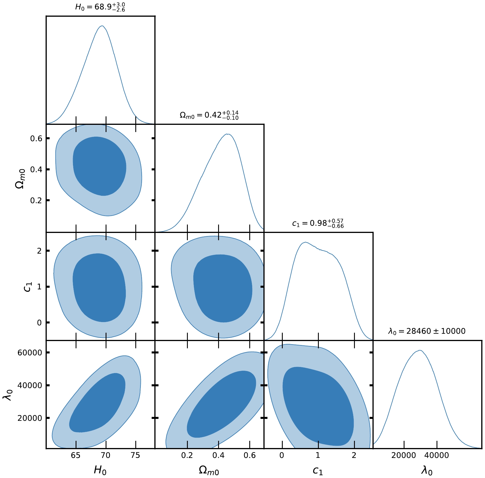
Figure 1. (color online) Contour plots of
$ H_{0}, \Omega_{m0}, c_{1}, \lambda_{0} $ at$ 1-\sigma $ and$ 2-\sigma $ confidence level in MCMC analysis of CC datasets for Model-I.
Figure 2. (color online) Contour plots of
$ H_{0}, \Omega_{m0}, \lambda, c_{2} $ at$ 1-\sigma $ and$ 2-\sigma $ confidence level in MCMC analysis of CC datasets for Model-II.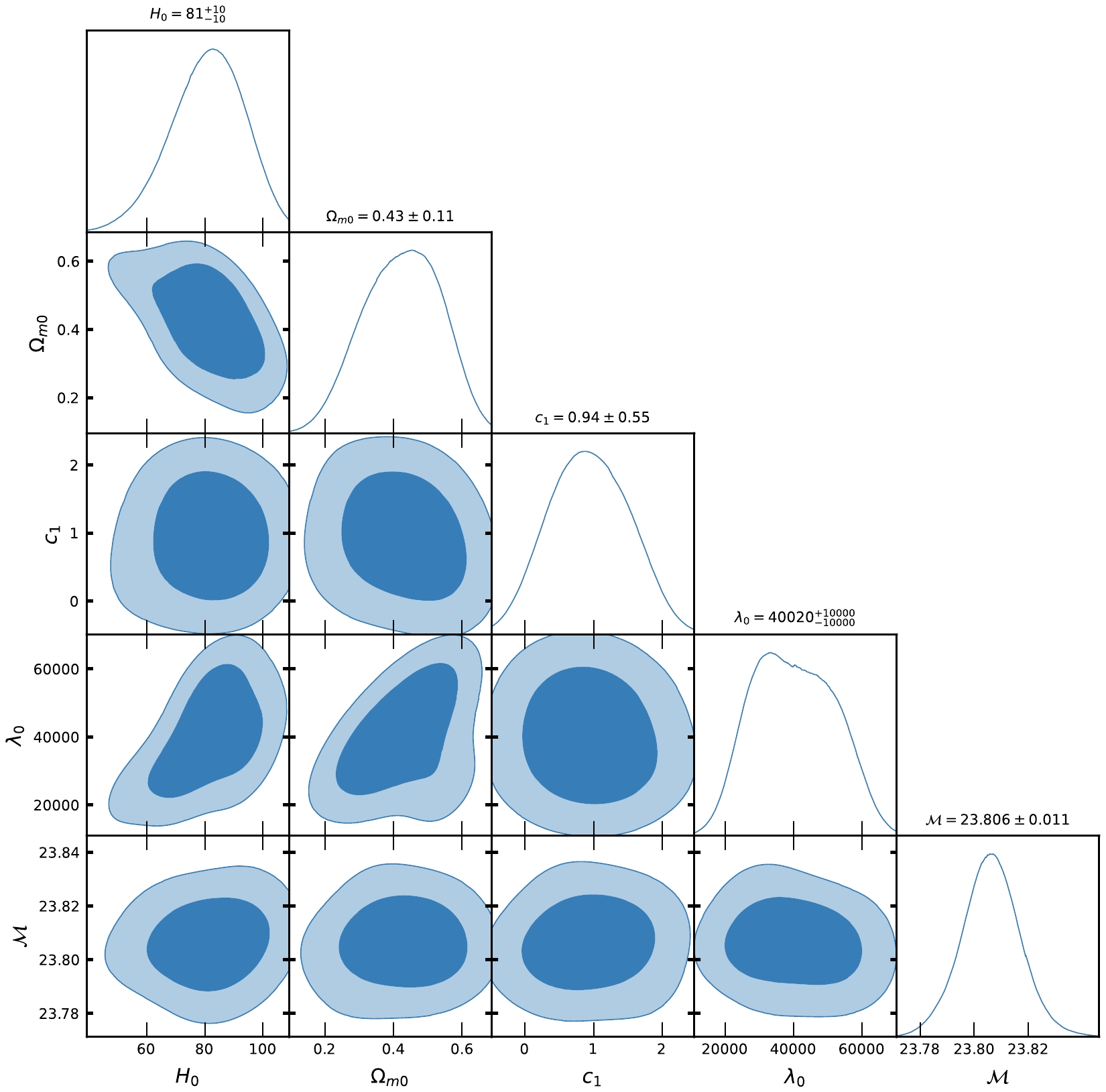
Figure 4. (color online) Contour plots of
$ H_{0}, \Omega_{m0}, c_{1}, \lambda_{0}, {\cal{M}} $ at$ 1-\sigma $ and$ 2-\sigma $ confidence level in MCMC analysis of Pantheon SNe Ia datasets for Model-I.
Figure 5. (color online) Contour plots of
$ H_{0}, \Omega_{m0}, \lambda, c_{2}, {\cal{M}} $ at$ 1-\sigma $ and$ 2-\sigma $ confidence level in MCMC analysis of Pantheon SNe Ia datasets for Model-II.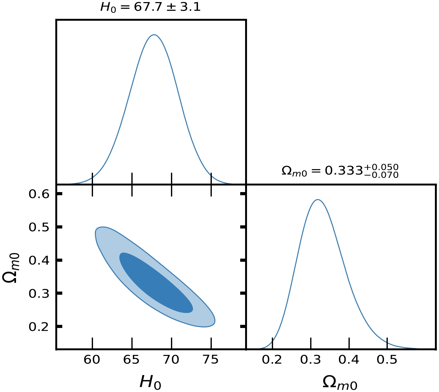
Figure 3. (color online) Contour plots of
$ H_{0}, \Omega_{m0} $ at$ 1-\sigma $ and$ 2-\sigma $ confidence level in MCMC analysis of CC datasets for ΛCDM.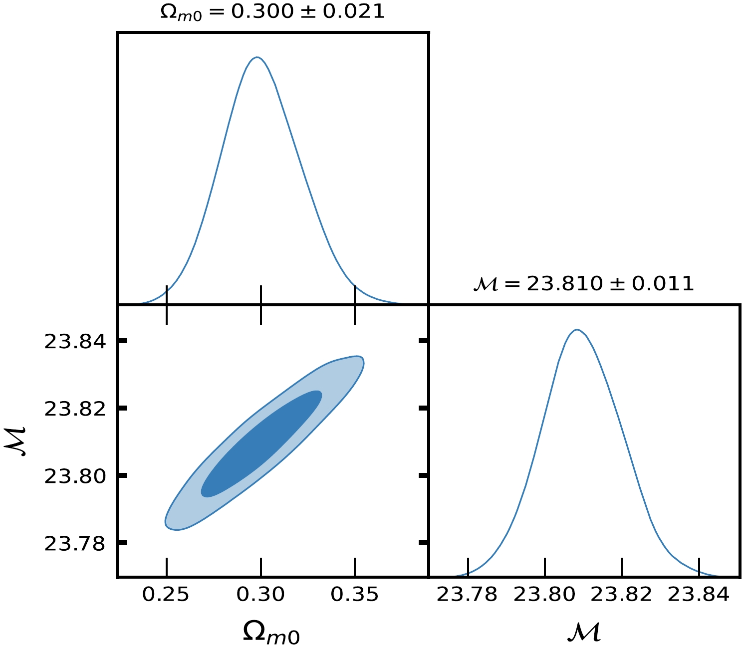
Figure 6. (color online) Contour plots of
$ H_{0}, \Omega_{m0}, {\cal{M}} $ at$ 1-\sigma $ and$ 2-\sigma $ confidence level in MCMC analysis of Pantheon SNe Ia datasets for ΛCDM.In the MCMC analysis of the CC
$ H(z) $ and Pantheon SNe Ia datasets for Model-I and Model-II, Figs. 1, 2, 4, and 5 show the contour plots of$ H_{0}, \Omega_{m0}, \lambda, \lambda_{0}, c_{1} $ and$ c_{2} $ at$ 1-\sigma $ and$ 2-\sigma $ confidence levels. Table 1 and Table 2 display the estimated values of cosmological parameters. The dimensionless parameter λ is constrained to an interval around$ 0 $ , which includes the ΛCDM paradigm. This was expected because, as we discussed above, a realistic modified gravity should present a small deviation from GR. Nevertheless, note that in both Model-I and Model-II, the λ-contours are slightly shifted towards positive values. To relax the degeneracy between the parameters λ,$ \lambda_{0} $ and$ c_{1}, c_{2} $ , we eliminated λ in Model-I and$ \lambda_{0} $ in Model-II. Recently, [71] estimated the value of$ \lambda = 0.491_{-0.533}^{+0.387}, 0.537_{-0.550}^{+0.403} $ , respectively, in two different models. The current values of the model parameter$ \lambda_{0} $ of dimension$ H_{0}^{2} $ are estimated as$ \lambda_{0} = 28460\pm10000, 40020\pm10000 $ along the two datasets. We estimated the approximate values of λ as$ \lambda = 0.417_{-0.398}^{+0.380}, 0.445_{-0.133}^{+0.099} $ for Model-I and$\lambda = 0.54\pm 0.28, 0.62_{-0.24}^{+0.30}$ for Model-II, along the two observational datasets, respectively.In the context of the estimated values of
$ \Omega_{m0} $ , we observed that Model-I and II give a rather large value due to the degeneracy with λ,$ \lambda_{0} $ and$ c_{1} $ ,$ c_{2} $ , whereas in ΛCDM, this is not the case. We determined the Hubble constant$ H_{0} $ for Model-I as$68.9_{-2.6}^{+3.0}, 81.0\pm10 \; {\rm{Km s^{-1} Mpc^{-1}}}$ , whereas for Model-II it was$68.3\pm2.6 \; {\rm{Km s^{-1} Mpc^{-1}}}$ , along the two datasets, respectively. For the ΛCDM, we obtained the value of the Hubble constant as$ H_{0} = 67.7\pm3.1 $ Km/s/Mpc. The values of$ H_{0} $ obtained in our estimation for Model-I and Model-II are large in comparison to ΛCDM due to the degeneracy with other parameters of the models. Recently, the present value of the Hubble constant was measured as$H_{0} = 69.8\pm1.3\; {\rm Km s^{-1} Mpc^{-1}}$ in [98] and$H_{0} = 69.7\pm1.2\; {\rm{Km s^{-1} Mpc^{-1}}}$ in [99]. This number was found to be$H_{0} = 66.6\pm1.6\; {\rm{Km s^{-1} Mpc^{-1}}}$ in [100] based on a large number of observational data. It was also found to be$H_{0} = 65.8\pm3.4\; {\rm{Km s^{-1} Mpc^{-1}}}$ in [101, 102]. The Hubble constant was measured as$H_{0} = 69.6\pm 0.8\; {\rm{Km s^{-1} Mpc^{-1}}}$ in [103],$H_{0} = 67.4_{-3.2}^{+4.1}\; {\rm{Km s^{-1}} {\rm{Mpc^{-1}}}}$ in [104],$H_{0} = 69_{-2.8}^{+2.9}\; {\rm{Km s^{-1} Mpc^{-1}}}$ in [105], and most recently,$H_{0} = 68.81_{-4.33}^{+4.99}\; {\rm{Km s^{-1}Mpc^{-1}}}$ in [106]. In 2018 , the Hubble constant was estimated by the Plank Collaboration to be$H_{0} = 67.4\pm0.5 \; {\rm{Km s^{-1} Mpc^{-1}}}$ , whereas in 2021, it was determined as$H_{0} = 73.2\pm1.3 \; {\rm{Km s^{-1} Mpc^{-1}}}$ in [107]. Recently, [108] estimated the value Hubble constant as$H_{0} = 69.504_{-0.141}^{+0.149} \; {\rm{Km s^{-1} Mpc^{-1}}}$ , [109] estimated it as$H_{0} = 68_{-2.0}^{+2.3} \; {\rm{Km s^{-1} Mpc^{-1}}}$ , whereas in [110], the value of the Hubble constant was reported as$H_{0} = 73.5\pm 1.1 \; {\rm{Km s^{-1} Mpc^{-1}}}$ for Pantheon+ datasets. When compared to previous results, the outcomes of our models I and II for$ H_{0} $ are consistent with observational datasets. For the two different models, we estimated the value of parameter$ {\cal{M}} = 23.806\pm0.011, 23.809\pm0.010 $ , whereas for ΛCDM, it was determined as$ {\cal{M}} = 23.810\pm0.011 $ . Recently, [111] estimated the value of$ {\cal{M}} = 23.809\pm0.013 $ .Equations (48) and (59) represent the expressions of
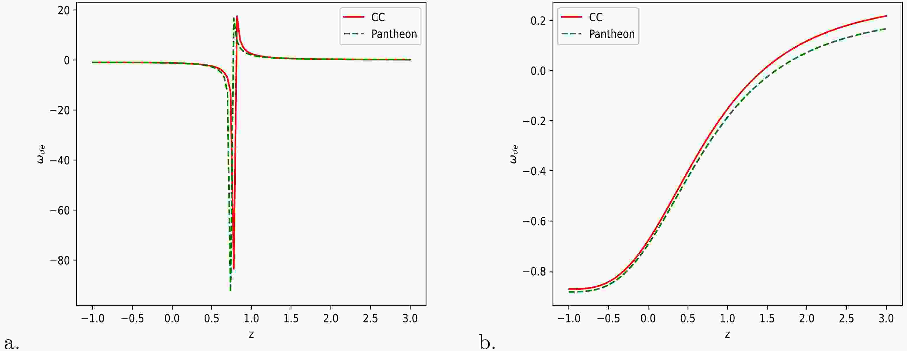
$ \omega_{de} $ for Model-I and Model-II, respectively. The variations of$ \omega_{de} $ over redshift z are depicted in Figs. 7 (a) and 7 (b), respectively, for Model-I and Model-II. From Fig. 7 (a), one can see that$\omega_{de} > -{1}/{3}$ for$ z_{t}>0.681, 0.678 $ for the two datasets, respectively, which corresponds to a decelerating expansion phase of the universe, whereas$\omega_{de} < -{1}/{3}$ over$-1 \leqslant z < 0.681,\; 0.678$ corresponds to the accelerating expansion phase of the universe. The lines$ z_{t} = 0.681, 0.678 $ show the phase transition line of the expanding universe with$\omega_{de} = -{1}/{3}$ . The present estimated values of$ \omega_{de} = -1.214_{-0.351}^{+0.206} $ for CC datasets and$ \omega_{de} = -1.233_{-0.182}^{+0.121} $ for Pantheon datasets are$ \omega_{de}\to-1 $ as$ z\to-1 $ . Figure 7 (b) shows that the dark energy EoS parameter$\omega_{de} > -{1}/{3}$ for transition redshifts$z_{t} = 0.626, 0.677$ along the two datasets used for Model-II, and$\omega_{de} < -{1}/{3}$ over$ -1\leqslant z <0.626, 0.677 $ along the same two datasets. The present value of$ \omega_{de} $ for Model-II is estimated as$ \omega_{de} = -0.679_{-0.006}^{+0.007} $ for CC datasets, and$\omega_{de} = -0.694_{-0.009}^{+0.006}$ along the Pantheon datasets, which corresponds to the accelerating phase of the expanding universe. In addition, we measured the late-time values of the EoS parameter as$ \omega_{de} = -0.872_{-0.053}^{+0.080}, -0.883_{-0.047}^{+0.099} $ along the two datasets, respectively. Thus, both Model-I and Model-II are transit phase (decelerating to accelerating) expanding universe models.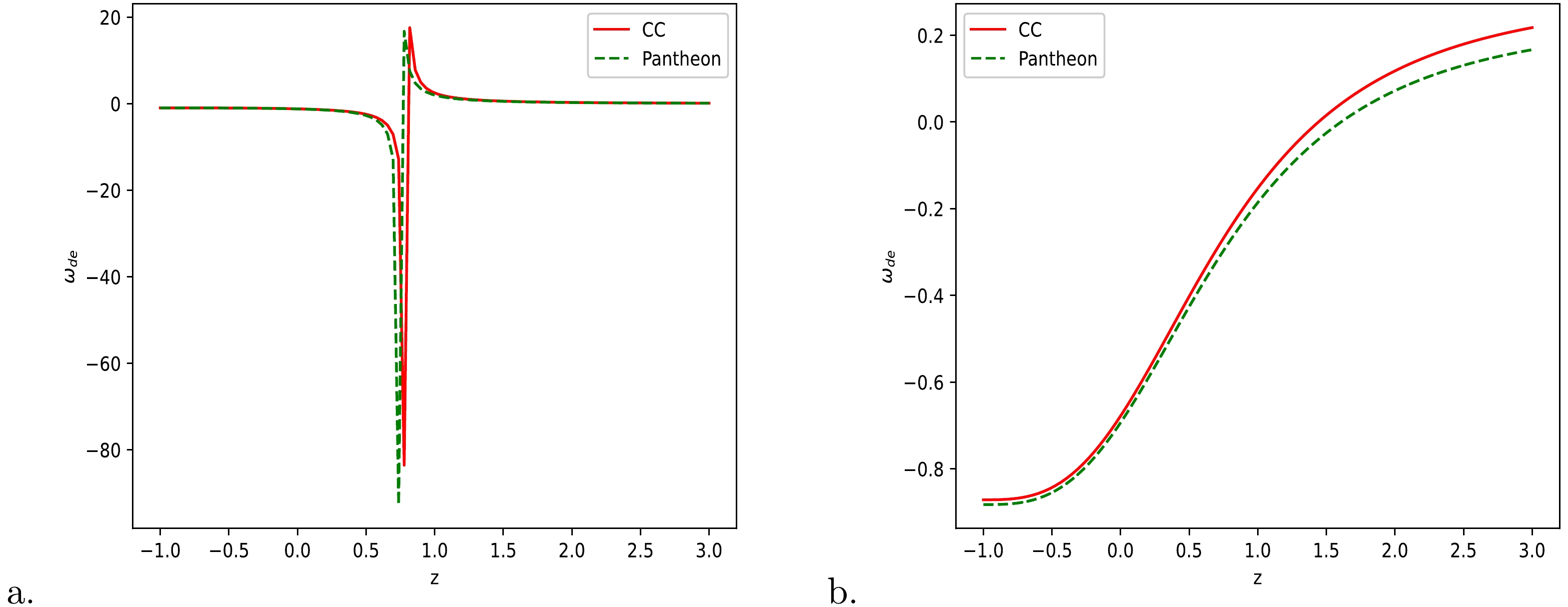
Figure 7. (color online) Variation of dark energy EoS parameter
$ \omega_{de} $ over redshift z for Model-I and Model-II, respectively.The expressions for the deceleration parameter
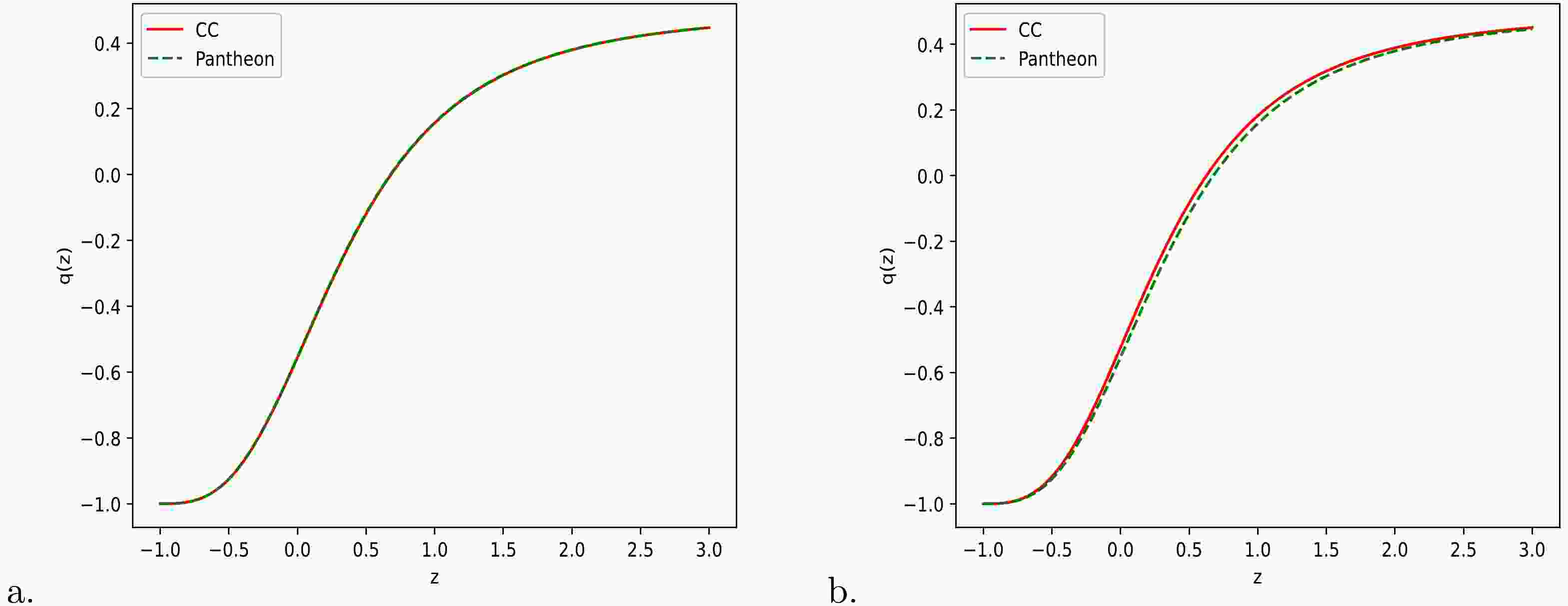
$ q(z) $ are represented by Eqs. (49) and (60), respectively, for models I and II. Figures 8 (a) and 8 (b), respectively, depict the geometrical evolution of$ q(z) $ for models I and II. From Figs. 8 (a) and 8 (b), it is clear that our two derived models are transit-phase universe models, which are decelerating in the past and accelerating in late-time scenarios. The transition redshift is measured as$z_{t} = 0.681, 0.678$ for Model-I and$ z_{t} = 0.626, 0.677 $ for Model-II along the two datasets, CC and Pantheon, respectively, and these values are consistent with recently observed values. The present value of the deceleration parameter is measured as$ q_{0} = -0.556, -0.554 $ for Model-I and$ q_{0} = -0.524, -0.553 $ for Model-II along the two datasets, respectively, which reveals the accelerating stage of the universe expansion. We obtain the relation$q = 0.5(1+3\omega_{de}\Omega_{de})$ for the models with dust fluid ($ p = 0 $ ), which gives the accelerating phase of the universe for$\omega_{de}\Omega_{de} < -{1}/{3}$ . Thus, for$ \Omega_{de} = 0 $ (i.e., for$ \rho_{de} = 0 $ ),$ q = 0.5>0 $ , we obtain a decelerating universe, and this confirms that the geometrical modification can explain the accelerating phase of an expanding universe.
Figure 8. (color online) Variation of deceleration parameter
$ q(z) $ over redshift z for Model-I and Model-II, respectively.From Table 3, we can observe that for the CC Hubble datasets, the AIC for both models is in the second group, with
$ 2<\Delta IC <6 $ . This means that our two derived models are in mild tension with the most popular ΛCDM, whereas the BIC is in the third group, with$ 6<\Delta IC <10 $ for Model-I and$ \Delta IC>10 $ for Model-II. This means that both models are in mild tension with ΛCDM [112]. Similarly, according to Table 4, for the Pantheon SNe Ia datasets, the AIC suggests that our two derived models are in mild tension with the most favored ΛCDM, whereas the BIC indicates that the models are strongly disfavored by the ΛCDM. -
We examined FLRW cosmological models within the framework of metric-affine
$ F(R,Q) $ gravity, as introduced in [84]. In this context, R represents the curvature scalar and Q represents the nonmetricity scalar, both calculated using non-special connections. The updated field equations were derived by employing a flat FLRW metric. In two distinct scenarios involving scalars u and w, we established a correlation between the Hubble constant$ H_{0} $ , density parameter$ \Omega_{m0} $ , and other model parameters. Subsequently, we employed recently acquired observational datasets, including the CC Hubble and the Pantheon SNe Ia datasets, to ascertain the most suitable values for the model parameters via MCMC analysis. By utilizing these optimal values of model parameters, we examined the outcomes and characteristics of the resulting models. Both of our models are transitional phase models and methods for the ΛCDM model in the late-time universe. We discovered that the geometric sector's dark equation of state parameter,$ \omega_{de} $ , exhibits similar behavior to that of a potential dark energy candidate.We considered two specific models, which are known to lead to interesting phenomenology. Our analysis shows that both models are capable of describing the evolution of the universe, supporting observational datasets, namely, CC Hubble data and Pantheon SNe Ia. We found a fairly large value of
$ \Omega_{m0} $ and a value of$ H_{0} $ that was between the Plank and local estimates but closer to the Plank estimate for both models, I and II, which both use the ΛCDM paradigm as a particular limit. For the dimensionless parameter λ, we constrained its value around 0, which shifted towards a positive value due to degeneracy with other parameters such as$ H_{0} $ and$ \Omega_{m0} $ . For the parameter$ \lambda_{0} $ dimensionally equivalent to Hubble constant$ H_{0}^{2} $ , we constrained its value around the value of the cosmological constant Λ.We investigated the behavior of the dark energy EoS parameter
$ \omega_{de} $ over z with constrained values of model parameters for both models. We observed that for Model-I, the present values of$ \omega_{de} $ fall in the range of phantom and super-phantom regions, whereas for Model-II, it falls into the quintessential region at late-time. We have also plotted the behavior of$ \omega_{de} $ with z in its value. The evolution of$ \omega_{de} $ is positive in the early universe for both models, and in late-time universe, it converts into negative values that are compatible with the evolution of the deceleration parameter$ q(z) $ , which depicts the expansion phase of the expanding universe. Model-I successfully reached the ΛCDM stage in the late-time universe, whereas Model-II shows quintessence scenarios at late-time. Finally, by applying the AIC and BIC, we determined that both Model-I and Model-II were less well-fitted with ΛCDM cosmological parameters. This is an interesting result because both Model-I and Model-II do not contain ΛCDM scenarios at present but depict the quintessence, phantom, and super-phantom scenarios. Both derived models are transit-phase accelerating universe models that can explain the late-time accelerating scenarios of the expanding universe.As this is the case, we showed that the
$ F(R,Q) $ gravity model can explain the accelerated phase of the expanding universe. The derived$ F(R,Q) $ gravity model's results are in mild tension with the ΛCDM standard cosmological model. Furthermore, the$ F(R,Q) $ gravity model allows us to recover the original Friedmann model. This$ F(R,Q) $ gravity theory is a generalization of both$ F(R) $ and$ F(Q) $ . As a result, the current modified gravity model is intriguing and attracts researchers to reexamine it in order to uncover other cosmological features of this$ F(R,Q) $ gravity theory. -
We are thankful to renowned referees and editors for their valuable suggestions to improve this manuscript.
FLRW cosmology in metric-affine F(R,Q) gravity
- Received Date: 2024-06-01
- Available Online: 2024-12-15
Abstract: We investigated some Friedmann-Lemaître-Robertson-Walker (FLRW) cosmological models in the context of metric-affine


 Abstract
 HTML
HTML Reference
 Related
 PDF
PDF




 DownLoad:
